
Top 15 Popular Machine Learning Metrics For Data Scientist
Machine learning is one of the most researched subjects of the last two decades. There is no end to human needs. But their production and working capability are limited. That’s why the world is moving towards automation. Machine Learning has a huge role in this industrial revolution. Developers are building more robust ML models and algorithms every day. But you cannot just throw your model into production without evaluating it. That’s where the machine learning metrics come in. Data scientists use these metrics to measure how good a model is predicting. You got to have a good idea about them. To make your ML journey convenient, we will be listing the most popular machine learning metrics you can learn to become a better data scientist.
Most Popular Machine Learning Metrics
We assume that you are well acquainted with the Machine Learning algorithms. If you are not, you can check our article about ML algorithms. Now let us go through the 15 most popular Machine Learning metrics you should know as a data scientist.
1. Confusion Matrix
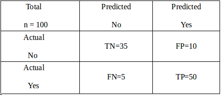
Data scientists use the confusion matrix to evaluate the performance of a classification model. It is actually a table. The rows depict the real value, whereas the columns express the predicted value. Since the evaluation process is used for classification problems, the matrix can be as big as possible. Let us take the example to understand it more clearly.

Suppose there are a total of 100 images of cats and dogs. The model predicted that 60 of them were cats, and 40 of them were not cats. However, in reality, 55 of them were cats, and the rest 45 were dogs. Assuming cats as positive and dogs as negative, we can define some important terms.
- The model predicted 50 cat images correctly. These are called True Positives (TP).
- 10 dogs were predicted to be cats. These are False Positives (FP).
- The matrix predicted correctly that 35 of them were not cats. These are called True Negatives (TN).
- The other 5 are called False Negatives (FN) as they were cats. But the model predicted them as dogs.
2. Classification accuracy
This is the simplest process to evaluate a model. We can define it as the total number of correct predictions divided by the total number of input values. In the case of the classification matrix, it can be said as the ratio of the sum of TP and TN to the total number of input.

Therefore, the accuracy in the above example is (50+35/100), i.e., 85%. But the process is not always effective. It may often give wrong info. The metric is most effective when the samples in each category are almost equal.
3. Precision and Recall
Accuracy doesn’t always work well. It may give wrong information when there is unequal sample distribution. So, we need more metrics to evaluate our model properly. That’s where precision and recall come in. Precision is the true positives to the total number of positives. We can know how much our model is responding in finding out the actual data.

The precision of the above example was 50/60, i.e., 83.33%. The model is doing well in predicting cats. On the other hand, recall is the ratio of true positive to the sum of a true positive and false negative. Recall shows us how often the model is predicting cat in the following example.

The recall in the above example is 50/55, i.e., 90%. In 90% of cases, the model is actually correct.
4. F1 Score
There is no end to perfection. Recall and precision can be combined to get a better evaluation. This is the F1 score. The metric is basically the harmonic mean of precision and recall. Mathematically it can be written as:

From the cat-dog example, the F1 Score is 2*.9*.8/(.9+.8), i.e., 86%. This is far more accurate than classification accuracy and one of the most popular Machine Learning metrics. However, there is a generalized version of this equation.

Using the beta, you can give more importance to either recall or precision; in the case of binary classification, beta=1.
5. ROC Curve
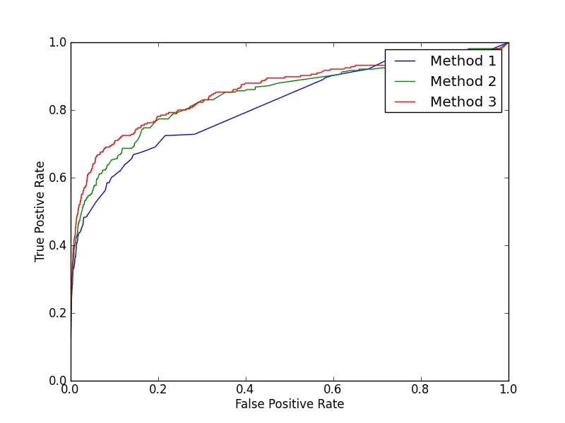
ROC curve or simply receiver operator characteristics curve shows us how our model works for different thresholds. In classification problems, the model predicts some probabilities. A threshold is then set. Any output bigger than the threshold is 1 and smaller than it is 0. For example, .2, .4,.6, .8 are four outputs. For threshold .5 the output will be 0, 0, 1, 1 and for threshold .3 it will be 0, 1, 1, 1.

Different thresholds will produce different recalls and precisions. This will eventually change the True Positive Rate (TPR) and False Positive Rate (FPR). ROC curve is the graph drawn by taking TPR on the y-axis and FPR on the x-axis. Accuracy gives us information about a single threshold. But ROC gives us a lot of thresholds to choose from. That’s why ROC is better than accuracy.
6. AUC
Area Under Curve(AUC) is another popular Machine Learning metrics. Developers use the evaluation process to solve binary classification problems. You already know about the ROC curve. AUC is the area under the ROC curve for various threshold values. It will give you an idea about the probability of the model choosing the positive sample over the negative sample.
AUC ranges from 0 to 1. Since FPR and TPR have different values for different thresholds, AUC also differs for several thresholds. With the increase in AUC value, the performance of model increases.
7. Log Loss
If you are mastering Machine Learning, you must know log loss. It is a very important and very popular Machine Learning metric. People use the process to evaluate models having probabilistic outcomes. Log loss increases if the model forecasted value diverges much from the real value. If the actual probability is .9 and the predicted probability is .012, the model will have a huge log loss. The equation for calculation log loss is as follows:

Where,
- p(yi)is the probability of positive samples.
- 1-p(yi) is the probability of negative samples.
- yi is 1 and 0 for positive and negative class, respectively.
From the graph, we notice that the loss decreases with increasing probabilities. However, it increases with a lower probability. Ideal models have 0 log loss.
8. Mean Absolute Error
Till now, we discussed the popular Machine Learning metrics for classification problems. Now we will be discussing the regression metrics. Mean Absolute Error (MAE) is one of the regression metrics. At first, the difference between the real value and the predicted value is calculated. Then the average of the absolutes of these differences gives the MAE. The equation for MAE is given below:

Where,
- n is the total number of inputs
- yj is the actual value
- yhat-j is the predicted value
The lower the error, the better is the model. However, you cannot know the direction of error because of the absolute values.
9. Mean Squared Error
Mean Squared Error or MSE is another popular ML metric. The majority of data scientists use it in regression problems. Like MAE, you have to calculate the difference between real values and predicted values. But in this case, the differences are squared, and the average is taken. The equation is given below:

The symbols indicate the same as MAE. MSE is better than MAE in some cases. MAE cannot show any direction. There is no such problem in MSE. So, you can easily calculate the gradient using it. MSE has a huge role in calculating gradient descent.
10. Root Mean Squared Error
This one is perhaps the most popular Machine Learning metric for regression problems. Root Mean Squared Error (RMSE) is basically the square root of MSE. It is almost similar to MAE except for the square root, which makes the error more precise. The equation is:

To compare it with MAE, let’s take an example. Suppose there are 5 actual values 11, 22, 33, 44, 55. And the corresponding predicted values are 10, 20, 30, 40, 50. Their MAE is 3. On the other hand, RMSE is 3.32, which is more detailed. That’s why RMSE is more preferable.
11. R-Squared
You can calculate the error from RMSE and MAE. However, the comparison between the two models is not exactly convenient using them. In classification problems, developers compare two models with accuracy. You need such a benchmark in regression problems. R-squared helps you to compare regression models. Its equation is as follows:

Where,
- Model MSE is the MSE mentioned above.
- Baseline MSE is the average of the square of differences between mean prediction and real value.
The range of R-square is from negative infinity to 1. The higher value of the evaluation means the model fits well.
12. Adjusted R-Squared
R-Squared has a drawback. It doesn’t act well when new features are added to the model. In that case, sometimes the value increases, and sometimes it remains the same. That means R-Squared doesn’t care if the new feature has anything to improve the model. However, this drawback has been removed in adjusted R-Squared. The formula is:

Where,
- P is the number of features.
- N is the number of inputs/samples.
In R-Squared Adjusted, the value only increases if the new feature improves the model. And as we know, the higher value of R-Squared means the model is better.
13. Unsupervised Learning Evaluation Metrics
You generally use the clustering algorithm for unsupervised learning. It is not like classification or regression. The model has no labels. The samples are grouped depending on their similarities and dissimilarities. To evaluate these clustering problems, we need a different type of evaluation metric. Silhouette Coefficient is a popular Machine Learning metric for clustering problems. It works with the following equation:

Where,
- ‘a’ is the average distance between any sample and other points in the cluster.
- ‘b’ is the average distance between any sample and other points in the nearest cluster.
The Silhouette Coefficient of a group of samples is taken as the average of their individual coefficients. It ranges from -1 to +1. +1 means the cluster has all points of the same attributes. The higher the score, the higher is the cluster density.
14. MRR
Like classification, regression, and clustering, ranking is also a Machine Learning problem. Ranking lists a group of samples and ranks them based on some particular characteristics. You regularly see this in Google, listing emails, YouTube, etc. Many data scientists keep Mean Reciprocal Rank (MRR) as their first choice for solving ranking problems. The basic equation is:

Where,
- Q is a set of samples.
The equation shows us how good the model is ranking the samples. However, it has a drawback. It only considers one attribute at a time to list items.
15. Coefficient of Determination (R²)
Machine Learning has a huge amount of statistics in it. Many models specifically need statistical metrics to evaluate. The coefficient of Determination is a statistical metric. It indicates how the independent variable affects the dependent variable. The relevant equations are:

Where
- fi is the predicted value.
- ybar is the mean.
- SStot is the total sum of squares.
- SSres is the residual sum of squares.
The model works best when =1. If the model predicts the mean value of data, will be 0.
Finally
Only a fool will put his model into production without evaluating it. If you want to be a data scientist, you must know about ML metrics. In this article, we have listed the fifteen most popular Machine Learning metrics that you should know as a data scientist. We hope you are now clear about different metrics and their importance. You can apply these metrics using Python and R.
If you study the article attentively, you should be motivated to learn the use of accurate ML metrics. We have done our job. Now, it’s your turn to be a data scientist. To err is human. There may be some lacking in this article. If you find any, you can let us know. Data is the new world currency. So, utilize it and earn your place in the world.


Leave a Reply